Adaptive 3-D Linear-Trajectory Filtering
Norm Bartley
3-D digital recursive filter algorithms based on
the simple 3-D inductance-resistance networks
are used to perform linear-trajectory filtering of
constant-velocity objects in image sequences. Using the same
3-D networks, we have designed adaptive 3-D recursive
filters, where the coefficients
of the filter are adapted on a frame-by-frame basis to track objects that
move on smooth, but nonlinear, trajectories. Such objects
are assumed to move on piece-wise linear trajectories.
Below are some input and output images from a contrived tracking
example.
We originally reported this work in 1986 in
this paper.
 At left is a single frame of a
computer-generated input sequence. This sequence contains two
objects that have intersecting helical trajectories. This is
shown in the
input MPEG sequence (16K, 100x100, 32 frames).
 The job is to lock onto and track
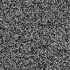
one of the above objects, and to exclude the other object. To add
challenge to the exercise, we add flat-spectrum noise at 10 times
the peak level of the objects. A single frame of the noisy sequence,
corresponding to the frame in the above input sequence,
is shown at left. Please play the
noise-contaminated MPEG
sequence (216K, 100x100, 32 frames),
and you will be hard-pressed to locate either object.
 Using an adaptive 3-D linear-trajectory
filter, we are able to suppress the noise and to track and enhance the object
of interest. As shown in the
output
MPEG sequence (21K, 100x100, 32 frames),
the object of interest has clearly been recovered from the noise and is
not affected by the object on the intersecting trajectory.
 The job is to lock onto and track
one of the above objects, and to exclude the other object. To add
challenge to the exercise, we add flat-spectrum noise at 10 times
the peak level of the objects. A single frame of the noisy sequence,
corresponding to the frame in the above input sequence,
is shown at left. Please play the
noise-contaminated MPEG
sequence (216K, 100x100, 32 frames),
and you will be hard-pressed to locate either object.
 At left is a single frame of a
computer-generated input sequence. This sequence contains two
objects that have intersecting helical trajectories. This is
shown in the
input MPEG sequence (16K, 100x100, 32 frames).
 Using an adaptive 3-D linear-trajectory
filter, we are able to suppress the noise and to track and enhance the object
of interest. As shown in the